Orbital Mechanics
In this excercise the two-body system of the Sun and Earth is used to compare the results of different integrators. The code is written in code units with the mass of the Sun, \(M\), being set to 1. With the mass of planet represented relative to the solar mass, the gravitational constant \(G\) can also be set to 1. The initial conditions for the position and velocity are given as 3-dimensional vectors on an XY plane. The necessary parameters can be set as follows:
import numpy as np

#capital letters = SUN, lower case = EARTH
M, m = 1.0, 3.0e-6

#Position vectors
X, x = np.array([0., 0., 0.]), np.array([1., 0., 0.])

#Velocity vectors
V, v = np.array([0., 0., 0.]), np.array([0., 1., 0.])
Different integrators are useful for different types of systems. For example, the fourth-order Hermite integrator is optimal for star cluster dynamics while symplectic integrators such as the Wisdom-Holman integrator are often used for secular evolution of planetary systems. The simplest integrator is the forward Euler integration scheme, which calculates the expected position and velocity of an object by assuming it drifts at a uniform velocity during a small time interval.
Euler Integrator
Below we demonstrate how to run the Euler integrator using different parameters.
The orbit object can be created using the orbit class, where \(dt\) and \(tend\) correspond to the timestep and the number of steps to take during the integration, respectively:
from AstroDynamics import orbits

#Integration parameters
dt, tend = 1e-3, 100

orbit = orbits.orbit(M=M, m=m, X=X, V=V, x=x, v=v, dt=dt, tend=tend, integrator='euler')
The plot_orbit method plots the position of the star and the planet in the x-y plane. The planet’s position is stored in the x_vec and y_vec attributes and the star’s position is stored in the X_vec and Y_vec attributes.
orbit.plot_orbit()
The calc_energy method calculates the energy of the system given the velocity and position vectors of the two celestial bodies. It calculates the magnitude of the velocity vectors, adds up the kinetic energy of both bodies, and subtracts the potential energy of the two bodies due to their mutual gravitational attraction. The method then saves the energy attribute which contains an array containing the energy of the system as a function of the integrated time. The plot_energy method can be used to plot the relative energy error of the system as a function of the time steps.
orbit.plot_energy()
The calc_momentum method calculates the angular momentum of the system given the velocity vectors and the separation distance between the two bodies. It uses the x and y components of the velocity vectors of the star, calculates the velocity of the planet relative to the star, and then calculates the \(\phi\) angle and angular velocity, after which the angular momentum is finally computed by multiplying the square of the separation distance and the angular velocity. The plot_momentum method plots the relative error in the angular momentum of the system as a function of the integration time steps.
orbit.plot_momentum()
We can change the integration parameters as need-be and re-configure the model:
orbit.tend = 1e4
orbit.m = 1e-3
orbit.x = np.array([0., 0., 1.])
orbit._run_()
Runge-Kutta
The Runge-Kutta methods are a family of numerical methods for approximating the solution of differential equations at every time step, with families of varying accuracy. The forward Euler method is a type of Runge-Kutta method of order one. The fourth-order Runge-Kutta method (RK4) is a common higher-order integrator. Runge-Kutta methods can be explicit or implicit. Implicit methods are more stable than explicit methods, but they require solving a system of algebraic equations. Multistep methods approximate the solution at each step using information from more than one previous step.
Plot the energy error up to 10 orbits for the Euler and RK4 integrators, using a timestep of 1e-2.
The integrator parameter can be set to either ‘euler’ or ‘runge-kutta’.
from AstroDynamics import orbits
import numpy as np

#capital letters = SUN, lower case = EARTH
M, m = 1.0, 3.0e-6
X = np.array([0., 0., 0.])
V = np.array([0., 0., 0.])
x = np.array([1., 0., 0.])
v = np.array([0., 1., 0.])

dt, tend = 1e-2, 10

euler = orbits.orbit(M=M, m=m, X=X, V=V, x=x, v=v, dt=dt, tend=tend, integrator='euler')
rk4 = orbits.orbit(M=M, m=m, X=X, V=V, x=x, v=v, dt=dt, tend=tend, integrator='runge-kutta')
The plot can be visualized as follows:
plt.plot(euler.timesteps, euler.energy_error, 'blue', marker = '*', label='Euler')
plt.plot(rk4.timesteps, rk4.energy_error, 'red', marker = 's', label='Runge-Kutta')
plt.xlabel('Time'), plt.ylabel(r'|$\Delta \rm E / \rm E_0|$')
plt.yscale('log')
plt.title('Error Growth')
plt.legend(prop={'size':14})
plt.show()

Plot the RK4 error in time, for different timesteps (10-1 to 10-4)
for timestep in [1e-1, 1e-2, 1e-3, 1e-4]:
    rk4 = orbits.orbit(M=M, m=m, X=X, V=V, x=x, v=v, dt=timestep, tend=tend, integrator='runge-kutta')
    plt.plot(rk4.timesteps, rk4.energy_error, label=r'$\Delta t$='+str(timestep))

plt.xlabel('Time'), plt.ylabel(r'|$\Delta \rm E / \rm E_0|$')
plt.yscale('log')
plt.title('Error Growth')
plt.legend(prop={'size':14})
plt.show()
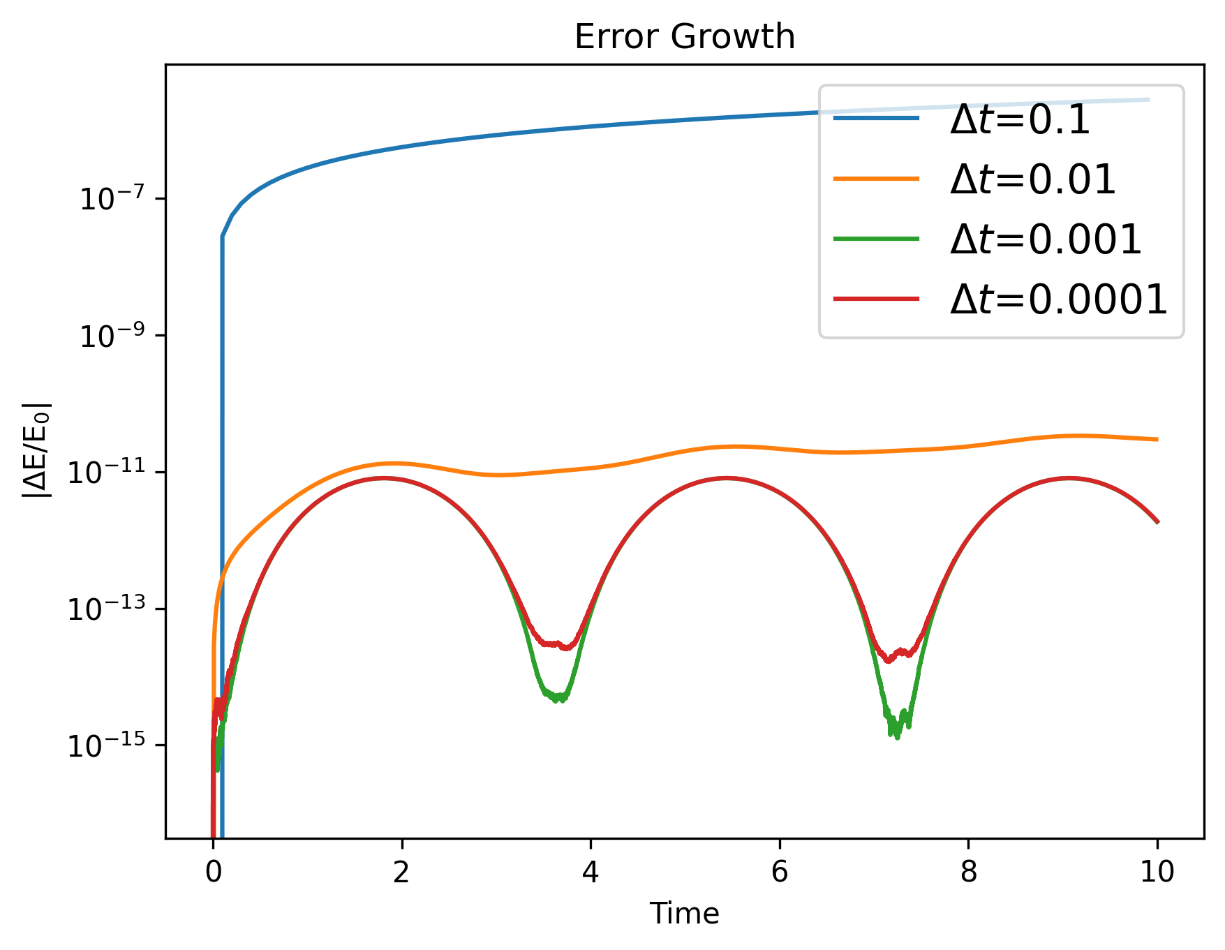
We can see that the error decreases with \(\Delta t^4\).
Leapfrog Integrator
The Euler method is a straightforward algorithm that approximates a numerical solution to an ordinary differential equation by using a simple forward-difference approximation of the derivative. In contrast, the leapfrog method (aka Kick-Drift-Kick (KDK)) is a more advanced integrator that works on second-order systems whose accelerations are not time-dependent. The leapfrog method propagates the position vectors and velocities at different times, while the Euler method propagates only the position vectors. The leapfrog method uses the value of the velocity at the midpoint of the time interval, whereas the Euler method takes the value of the velocity at the beginning of the interval. Finally, the leapfrog method is symplectic, which means that it preserves the Hamiltonian nature of the system being modeled.
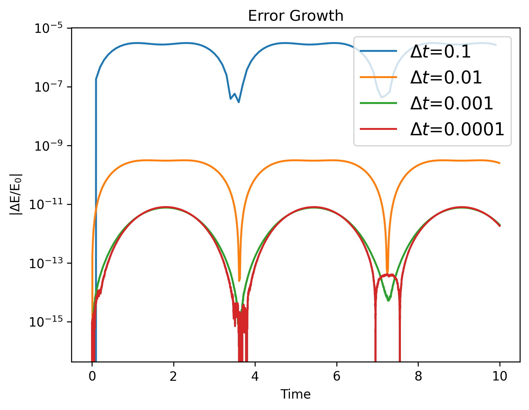
Compare the error with KDK for different timesteps, up to 10 orbits
We can set the integrator parameter to ‘leapfrog’:
from AstroDynamics import orbits
import matplotlib.pyplot as plt
import numpy as np

#capital letters = SUN, lower case = EARTH
M, m = 1.0, 3.0e-6
X = np.array([0., 0., 0.])
V = np.array([0., 0., 0.])
x = np.array([1., 0., 0.])
v = np.array([0., 1., 0.])
tend = 10

for timestep in [1e-1, 1e-2, 1e-3, 1e-4]:
    lf = orbits.orbit(M=M, m=m, X=X, V=V, x=x, v=v, dt=timestep, tend=tend, integrator='leapfrog')
    plt.plot(lf.timesteps, lf.energy_error, label=r'$\Delta t$='+str(timestep))

plt.xlabel('Time'), plt.ylabel(r'|$\Delta \rm E / \rm E_0|$')
plt.yscale('log')
plt.title('Error Growth')
plt.legend(prop={'size':14})
plt.show()
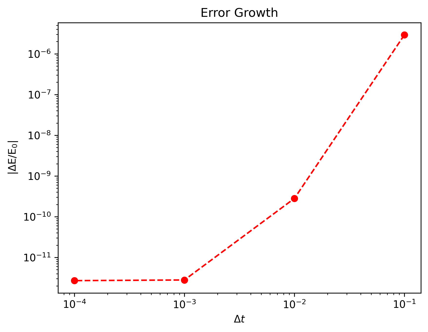
Plot the error after one orbit, what is the order of the integrator?
tend = 1
timesteps, errors = [],[]
for timestep in [1e-1, 1e-2, 1e-3, 1e-4]:
    lf = orbits.orbit(M=M, m=m, X=X, V=V, x=x, v=v, dt=timestep, tend=tend, integrator='leapfrog')
    timesteps.append(timestep), errors.append(lf.energy_error[-1])

plt.plot(timesteps, errors, 'ro--')
plt.xlabel(r'$\Delta t$'), plt.ylabel(r'|$\Delta \rm E / \rm E_0|$')
plt.yscale('log'), plt.xscale('log')
plt.title('Error Growth')
plt.show()
Compare the error for timestep=1e-3 for Euler, RK4, and KDK.
dt, tend = 1e-3, 10

for integrator in ['euler', 'runge-kutta', 'leapfrog']:
    orbit = orbits.orbit(M=M, m=m, X=X, V=V, x=x, v=v, dt=dt, tend=tend, integrator=integrator)
    plt.plot(orbit.timesteps, orbit.energy_error, label=integrator)

plt.xlabel('Time'), plt.ylabel(r'|$\Delta \rm E / \rm E_0|$')
plt.yscale('log')
plt.title('Error Growth')
plt.legend(prop={'size':14})
plt.show()

Excercises
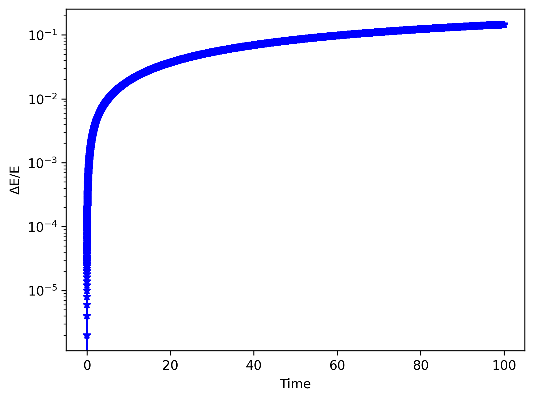
(1) Use \(\Delta\) t = 1e-3, up to t = 100. Plot the energy error in log, against time.
import numpy as np
from AstroDynamics import orbits

#capital letters = SUN, lower case = EARTH
M, m = 1.0, 3.0e-6
X = np.array([0., 0., 0.])
V = np.array([0., 0., 0.])
x = np.array([1., 0., 0.])
v = np.array([0., 1., 0.])

dt = 1e-3
tend = 100.

orbit = orbits.orbit(M=M, m=m, X=X, V=V, x=x, v=v, dt=dt, tend=tend, integrator='euler')
orbit.plot_energy()
(2) Plot the angular momentum error vs time.
orbit.plot_momentum()

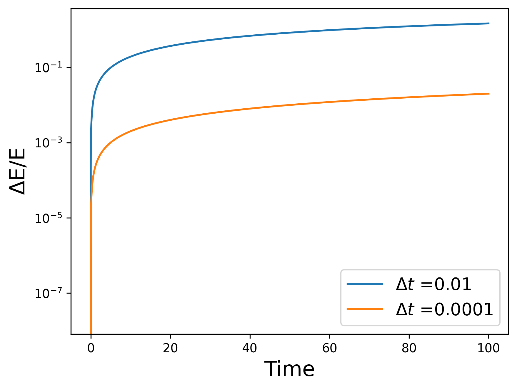
(3) Compare the energy error vs time for the run above, with runs using \(\Delta\) t = 1e-4, and \(\Delta\) t = 1e-2. Explain the trend.
The smaller the timestep, the lower the error! This is because the Euler integrator assumes a constant velocity over each timestep. Since velocities aren’t constant over the timestep, the smaller timestep results in less error.
import matplotlib.pyplot as plt

for dt in [1e-2, 1e-4]:
    orbit.dt = dt
    orbit._run_()
    plt.plot(orbit.timesteps, orbit.energy_error, label=r'$\Delta t$ ='+str(dt))

plt.xlabel('Time', size=17), plt.ylabel(r'$\Delta \rm E / \rm E$', size=17)
plt.yscale('log')
plt.legend(prop={'size':14})
plt.show()
(4) Plot the energy error after 1 orbit for three different timesteps: 1e-4, 1e-3, 1e-2.
orbit.tend = 1.0

for timestep in [1e-4, 1e-3, 1e-2]:
    orbit.dt = timestep
    orbit._run_()
    plt.plot(np.arange(0, orbit.tend, orbit.dt), orbit.energy_error, label=r'$\Delta t$='+str(timestep))

plt.xlabel('Time', size=17), plt.ylabel(r'$\Delta \rm E / \rm E$', size=17)
plt.yscale('log')
plt.legend(prop={'size':14})
plt.show()

(5) Time the code with the acceleration given by \(\frac{r_{vec}}{r^3}\) vs \(\frac{r_{hat}}{r^2}\). State the performance in microseconds per timestep.
The class instance contains the approx attribute which determines whether the acceleration is approximated as one over \(r^3\) or whether it’s calculated as the unit vector divided by \(r^2\).
r2, r3 = [],[]
for timestep in [1e-4, 1e-3, 1e-2]:
    orbit.dt = timestep
    orbit.approx = True
    orbit._run_()
    r3.append(orbit.integration_time*1e6/len(orbit.timesteps))
    orbit.approx = False
    orbit._run_()
    r2.append(orbit.integration_time*1e6/len(orbit.timesteps))

plt.plot([1e-4, 1e-3, 1e-2], r2, 'ro-', label=r'$\frac{1}{r^2}$')
plt.plot([1e-4, 1e-3, 1e-2], r3, 'b*--', label=r'$\frac{1}{r^3}$')
plt.xlabel(r'$\Delta t$', size=17), plt.ylabel(r'$\mu s$ / $\Delta t$', size=17)
plt.legend(prop={'size':14})
plt.show()

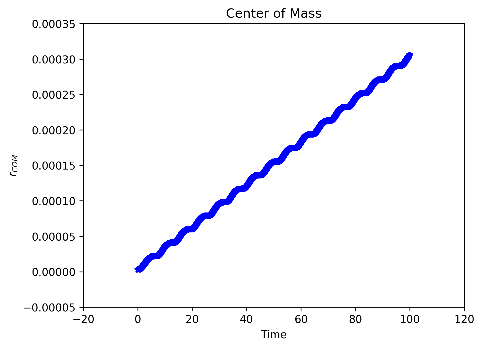
(6) Plot the position and velocity of the center of mass, against time.
orbit.plot_com()
orbit.plot_vcom()

(7) How would you modify your code to eliminate the evolution of the center of mass?
To eliminate the evolution of the center of mass and constrain it to the origin of the system’s frame, the center of mass’ position vector should be subtracted from both the Earth and Sun’s position vectors shifting the system toward the Sun.